Weighted correlation between weighted averaging optima and constrained ordination species scores.

obs.cor calculates the weighted correlation between the species weighted average optima and the axis one species scores of an ordination constrained by the WA reconstruction.

Usage

obs.cor(
  spp,
  env,
  fos,
  ord = rda,
  n = 99,
  min.occur = 1,
  autosim,
  permute = FALSE
)

# S3 method for class 'obscor'
plot(
  x,
  xlab,
  ylab,
  f = 5,
  which = 1,
  variable_names = "env",
  abun = "abun.calib",
  p_val = 0.05,
  ...
)

# S3 method for class 'obscor'
identify(x, labels, ...)

# S3 method for class 'obscor'
autoplot(
  object,
  which = 1,
  variable_names = "env",
  abun = "abun.calib",
  p_val = 0.05,
  nbins = 20,
  top = 0.7,
  ...
)

Arguments

spp: Data frame of modern training set species data, transformed if required, for example with sqrt
env: Vector of a single environmental variable
fos: Data frame of fossil species data. Species codes and transformations should match those in spp.
ord: Constrained ordination method to use. rda is the default, cca should also work. capscale won't work without modifications to the code (or a wrapper).
n: number of random training sets. More is better.
min.occur: Minimum number of occurrences of species in the species and fossil data.
autosim: Optional data frame of random values. This is useful if the training set is spatially autocorrelated and the supplied data frame contains autocorrelated random variables. If autosim is missing, and permute is FALSE, the transfer functions are trained on random variables drawn from a uniform distribution.
permute: logical value. Generate random environmental variables by permuting existing variable. Only possible if there is only one environmental variable and autosim is missing.
x: An obscor object.
xlab: X-axis label if the default is unsatisfactory.
ylab: Y-axis label if the default is unsatisfactory.
f: Scale factor for the abundances, the maximum cex of points for the which=1 plot.
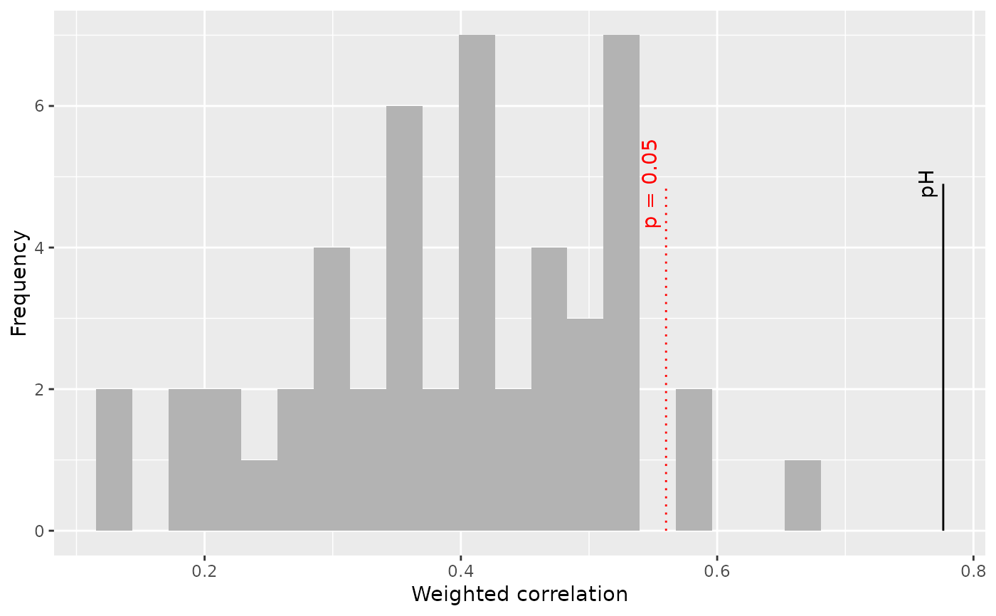
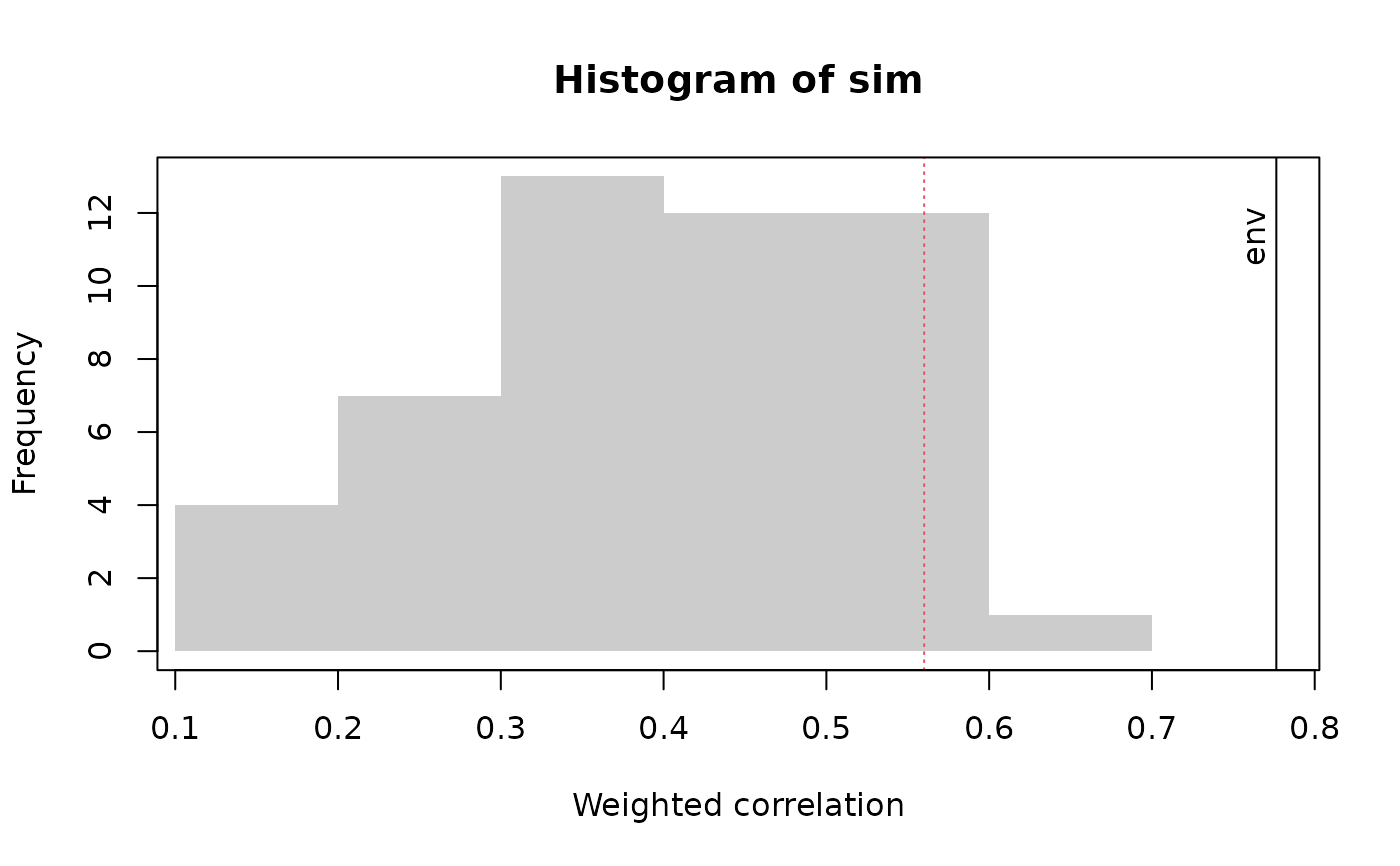
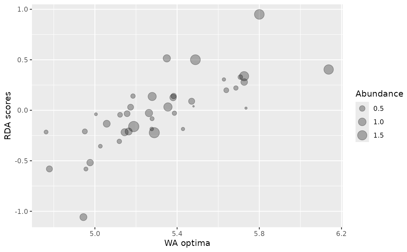
which: Which type of plot. which = 1 gives a plot of RDA scores against species optima. which = 2 gives a histogram showing the null distribution of correlations between RDA scores and species optima, together with the observed correlation.
variable_names: Name of environmental variable (only 1 currently) for the label on the observed correlation with which = 2
abun: Which species weighting required for plots. See details
p_val: P value to draw a line vertical line at (with which=2)
...: Other arguments to plot or identify
labels: Labels for the points in identify. By default, the species names from intersection of colnames(spp) and colnames(fos) are used.
object: An obscor object.
nbins: integer giving number of bins for the histogram
top: Proportion of the figure below the environmental name labels.

Value

obs.cor returns an obscor object, which is a list

ob: Observed correlation. Data.frame with columns Optima, RDA1 and abun containing the species optima, ordination axis 1 scores, and abundance used to weight the species respectively and a vector containing the weighted and unweighted correlations between species optima and ordination scores.
sim: Matrix with the correlation between species weighted average optima and ordination scores in the first column and the weighted correlation in the second column. Each row represents a different random environmental variable.
sigs: p-value for the observed correlation between species weighted average optima and ordination scores for each of the weights.

Details

Obs.cor calculates the (weighted) correlation between the species WA optima in the calibration set and their ordination axis one scores in the fossil data. Seven different weights for the species are implemented.

"abun.fos" - weight by the mean abundance in the fossil data.
"abun.calib" - weight by the mean abundance in the calibration data
"abun.joint" - weight by the product of the mean abundance in the fossil and calibration data
"n2.fos" - weight by the effective number of occurrences (Hill's N2) of each species in the fossil data
"n2.calib" - weight by the effective number of occurrences (Hill's N2) of each species in the calibration data
"n2.joint" - weight by the product of n2.calib and n2.fos
"unweighted" - all species receive same weight. This is unlikely to be the best option but is included for completeness.

It is unclear which of these weights is likely to be best: research is in progress. A square root transformation of the species data is often useful. n = 99 is too small in practice to give a smooth histogram of the null model. n = 999 is better.

Functions

plot(obscor): Plots for obscor object
identify(obscor): Identify species on obs.cor plot
autoplot(obscor): autoplot for obscor object

Note

The test of the weighted correlation between species optima and ordination axis scores is more powerful, especially with a small number of fossil observations, that the test of variance explained in randomTF but is only applicable to WA and will have a large type II error if there are few species.

References

Telford, R. J. and Birks, H. J. B. (2011) A novel method for assessing the statistical significance of quantitative reconstructions inferred from biotic assemblages. Quaternary Science Reviews 30: 1272–1278. doi:10.1016/j.quascirev.2011.03.002

Author

Richard Telford richard.telford@uib.no

Examples

require(rioja)
data(SWAP)
data(RLGH)
rlgh.obs <- obs.cor(
  spp = sqrt(SWAP$spec),
  env = SWAP$pH,
  fos = sqrt(RLGH$spec),
  n = 49 # low number for speed
)
rlgh.obs$sig
#>   abun.fos abun.calib abun.joint     n2.fos   n2.calib   n2.joint unweighted 
#>       0.02       0.02       0.02       0.02       0.02       0.02       1.00 
plot(rlgh.obs, which = 1)

plot(rlgh.obs, which = 2)


require(ggplot2)
#> Loading required package: ggplot2
autoplot(rlgh.obs, which = 1)

autoplot(rlgh.obs, which = 2, variable_names = "pH")